Path integral Monte Carlo

Introduction

The path integral Monte Carlo (PIMC) approach is a numerical finite temperature method that can treat systems with just a few number of particles to hundreds of particles. It has been widely applied to many different areas of physics such as condensed matter systems, nanowires, van der Waals clusters, quantum dots, nuclear matter, cold atoms, etc. Superfluidity of bulk helium, e.g., was first numerically confirmed using PIMC techniques. Many other thermodynamic quantities of bosonic systems such as the internal energy, heat capacity, density distribution, and pair correlation function can also be calculated exactly. Even though only Bose statistics has been widely treated in the literature, it is also possible to treat systems with Fermi statistics. At low temperature, the Fermi sign problem makes the simulations demanding, but we can, at least for certain fermionic systems, treat temperatures near or in the quantum degenerate regime without “hitting” the sign problem.

Below we give a simple example of a PIMC calculation for a single particle in a harmonic trap.

Single particle in the harmonic trap - the eigen state basis

For a single particle in a harmonic trap described by the Hamiltonian $\mathcal{H}$,

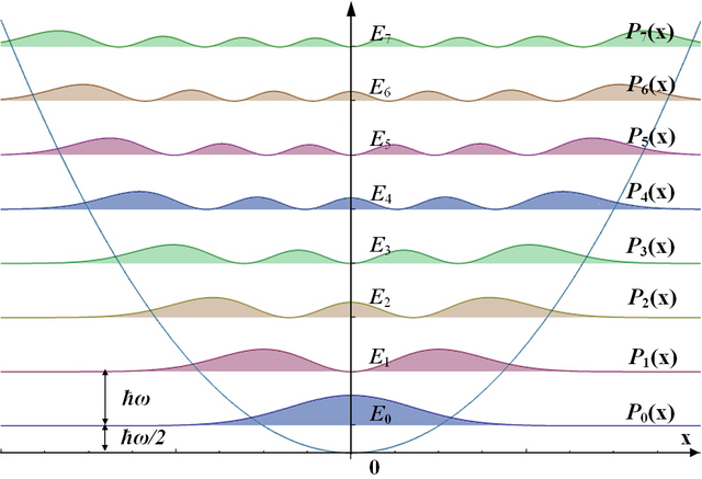
\[\mathcal{H}=-\frac{\hbar^2}{2m}\frac{\partial^2}{\partial x^2}+\frac{1}{2}m \omega^2 x^2,\]

where $\hbar$, $m$, and $\omega$ are the reduced Planck’s constant, the mass of the particle, and the angular trapping frequency, respectively, we can calculate the eigen energies $E_j$ and eigen functions $\psi_j$. The thermal average over all the allowed states with the Boltzmann weight $e^{-E_j/k_BT}$, where $k_B$ is the Boltzmann constant and $T$ the temperature, yields the finite temperature properties. While the single particle harmonic oscillator problem is simple enough that this “brute force” approach is possible, it becomes much harder or even impossible if we consider two, three,… particles with interactions. The figure on the left, adopted from Wikipedia, illustrates the eigen values and square of the eigen functions for a single particle in the harmonic trap.

Density matrix and Trotter formula

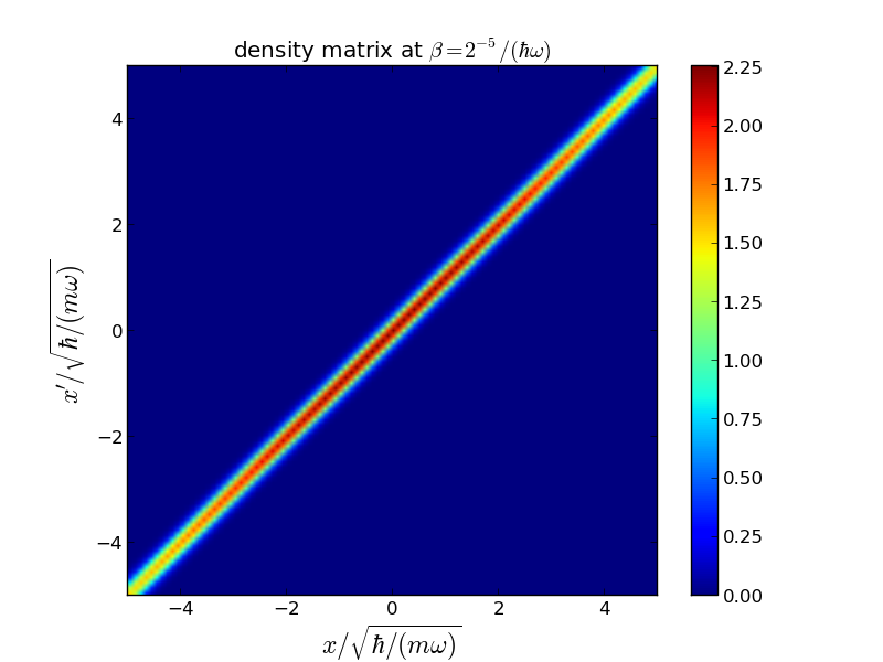
Now we introduce the path integral method that accounts the finite temperature. The density matrix $\rho(x,x',\beta)$, $\rho(x,x',\beta)=\bra{x}\exp(-\beta \mathcal{H})\ket{x'},$ where $\beta=1/(k_BT)$ is the inverse temperature (or “imaginary time”), is the key quantity from which we can calculate almost every thermodynamic observable that we are interested in. The Trotter formula reads $e^{-\beta (\mathcal{K}+\mathcal{V})}= e^{-\beta\mathcal{V/2}}e^{-\beta\mathcal{K}}e^{-\beta\mathcal{V/2}} +O(\beta^3),$ where $\mathcal{K}$ and $\mathcal{V}$ are the kinetic energy and potential energy operators. The density matrix can be approximated fairly accurately at high temperature but not, in general, at low temperature. The figure on the left shows the density matrix at a relatively high temperature, i.e., at $\beta=\frac{1}{32}\hbar\omega$.

Convolution of the density matrix

Using the convolution property of the density matrix,

\[\rho(x_0,x_2,\beta)=\int dx_1 \rho(x_0,x_1,\beta/2)\rho(x_1,x_2,\beta/2),\]

we can express the density matrix at low temperature (small $\beta$) as a product of two density matrices at higher temperature (large $\beta$). The price to pay is an additional integration over $x$. Another way of understanding this is to insert a complete set of position basis:

\[\rho(x_0,x_2,\beta)=\int dx_1 \bra{x_0}\exp(-\beta \mathcal{H}/2)\ket{x_1}\bra{x_1}\exp(-\beta \mathcal{H}/2)\ket{x_2}.\]

To get accurate simulation results, we have to insert sufficiently many intermediate position basis, i.e., we have to perform sufficiently many “auxiliary integrations”,

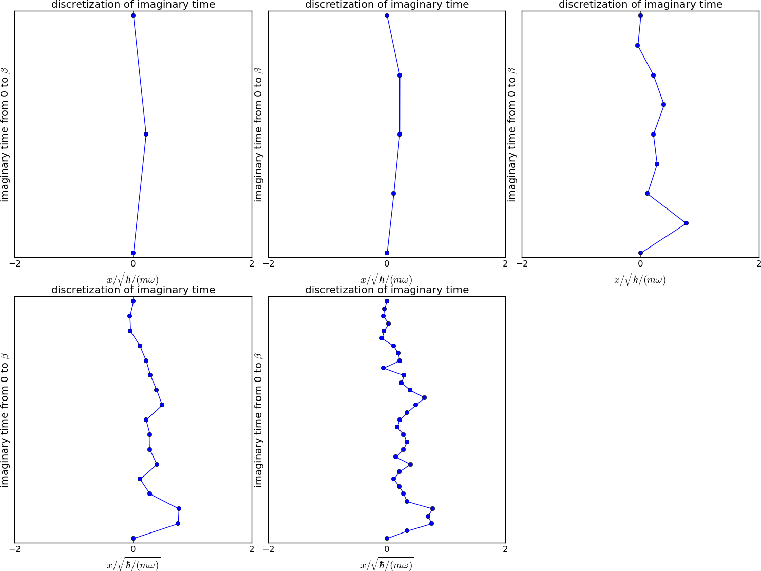
\[\rho(x_0,x_M,\beta)=\int dx_1\dots\int dx_{M-1} \bra{x_0}\exp(-\beta \mathcal{H}/M)\ket{x_1}\dots\\\bra{x_{M-1}}\exp(-\beta \mathcal{H}/M)\ket{x_M}.\]

The number of time slices $M$ depends on the desired accuracy. The figure on the left illustrates the discretization of the imaginary time. The dots and the links represent the position bases and the density matrices, respectively. In the last plot, $M$ is 32, i.e., we inserted 31 intermediate points. The multi-dimensional integral can be evaluated using Monte Carlo techniques.

Naive path integral Monte Carlo

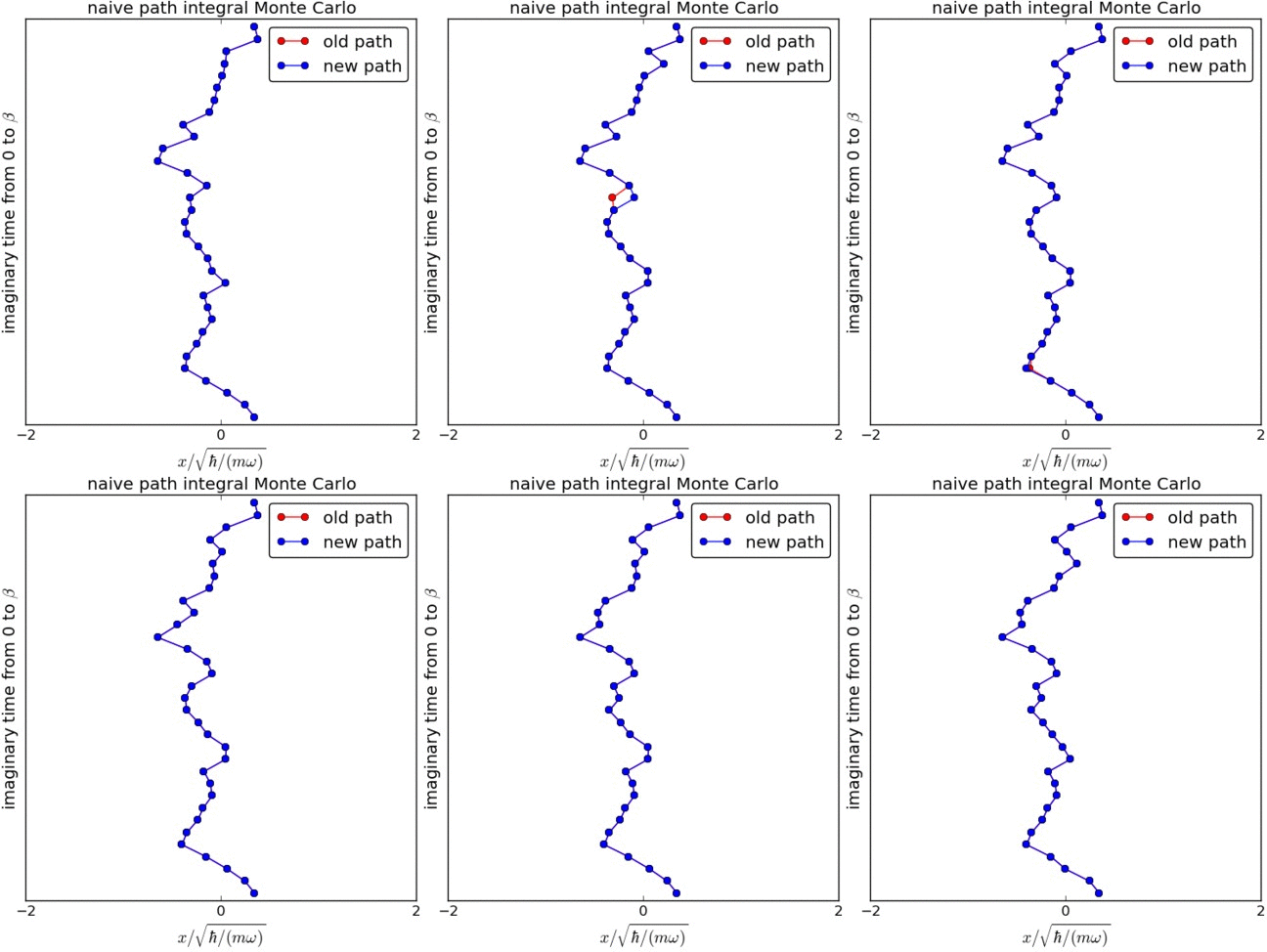
To calculate the density distribution of the particle, we only need the diagonal elements of the density matrix. This corresponds to $x_M=x_0$, i.e., the path is closed and can be thought of as a ring. We sample the path using a Markov chain. To update the path, we calculate the ratio $p$ of the density matrices represented by the proposed new path and those represented by the old path. The probability of accepting the path is determined by $p$ ($p$ if $p<1$, 1 if $p\geq1$). A naive way of constructing a proposed new path is to move a single “bead” as illustrated in the figure on the left. We note that there is a finite probability that the proposed new path is rejected, which implies that the bead stays at its position. This naive update method suffers from long correlation times and is, in general, not used in state-of-the-art simulations.

Multilevel path integral Monte Carlo

A smarter way to construct a proposed new path is to move several consecutive “beads”, i.e., a segment of the path simultaneously. This approach is commonly referred to as multilevel PIMC approach. The figure on the left illustrates the multilevel PIMC method.

Density distribution

Finally, from the simulated paths, we can extract the observables that we are interested in. We choose the density distribution function to illustrate the procedure. The density is simply the distribution of the $x$ position that we plotted in the figures above. We get the density distribution function by collecting the position values as the simulation goes on. The figure on the left shows the histogram of the position, i.e., the density distribution.

Summary

The above movies/figures illustrate the basic idea of the PIMC technique for a single particle in a harmonic trap. It is important to realize that the PIMC technique can do much more. We can simulate many particles with specified statistics and with arbitrary interactions including two-body interactions and three-body interactions. Examples of our results obtained by the PIMC approach can be found in the following references:
Y. Yan and D. Blume, JPB 50, 223001 (2017)
Y. Yan and D. Blume, PRL 112, 235301 (2014)
Y. Yan and D. Blume, PRA 88, 023616 (2013)

Further read

“Statistical Mechanics: Algorithms and Computations” by Werner Krauth (see coursera).